Guide to Experiment 2: Diodes
Métodos da Físcia Experimental I: (F540 2s2020)
JupyterBook: Gustavo Wiederhecker, Varlei Rodrigues
Contributions: Daniel Ugarte, Antônio Riul Junior, Varlei Rodrigues
In this experiment, the role of diodes in electric circuits will be investigated. A diode is a nonlinear elementcomposed of a semiconductor junction with different doping of the p and n type, a pn junction. This junction allows the passage of a high current \( (\approx 1 A) \) when directly polarized and very low \( (\approx 10 ^ {- 5} A) \) when it is reverse polarized.
To fully appreciate this device, it is desirable that you read an introductory text on the band theory of solids (Sections 3.1.1 to 3.1.4 in [1]). Then, you should recap the method of load-lines to solve Kirchhoff’s law when a diode is present, as section 3.2.1 in [1].
Goals
Understand the behavior and simple applications of a diode in a circuit.
Build a DC voltage source using a diode as the rectifying element.
Items to include in your lab report
Graphs of the time-traces corresponding two different load conditions (resistance values). You must generate the graphs, based on the data provided in Downloadable dataset 1.
Try to add the different traces to a single figure, instead of adding multiple repetitive plots to your report. Consider distinct line colors for each trace.
Extract the following parameters from each plots
Average voltage
Ripple voltage
RMS voltage
Compare the extracted ripple data with (15) and (16). Can you extract the capacitance from this model?
Provide hyperlinks to your TinkerCAD simulation and upload your QUCS file.
#-----------------------------
#Pacote para manipular vetores e matrizes
import numpy as np
import pandas as pd
#-----------------------------
#Pacotes para lidar com unidades
from astropy import units as un
from astropy import constants as cte
#-----------------------------
#pacote para gráficos
import matplotlib.pyplot as plt
import matplotlib
#Comandos opcionais para formatar gráfico
font = {'family' : 'Arial',
        'weight' : 'normal',
        'size'   : 12}
lines = {'linewidth' : 3.0}
figure = {'figsize' : [6.0, 6/1.6]}
matplotlib.rc('font', **font)
matplotlib.rc('lines', **lines)
matplotlib.rc('figure', **figure)
#-----------------------------
from myst_nb import glue
#pacote para desenhar circuitos
import SchemDraw as schem
import SchemDraw.elements as e
d = schem.Drawing(unit=2.5) # unit=2.5 determina o tamanho dos componentes
# %config InlineBackend.figure_format = 'svg'
Diode current-voltage curves (I-V curve)
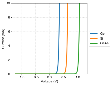
Consider a circuit containing an element whose relationship between voltage and current is non-linear, for example, a diode. The diode case provides an important application of the load curve method mentioned above. When breakdown(see section 3.1.5 in [1]) effects are ignored, the current-voltage relation in a diode is given by the Schockley equation,
where,
\(I_S\) [A] reverse saturation current ;
\(k_B\approx1.38\times10^{-23} \) [J/K] is the Boltzmann constant;
\(T \) [K] is the pn junction temperature;
\(q\approx1.6\times 10^{-19} \) [C] is the electron charge.
Note that \(q/(k_B T)\approx39.6\equiv \beta \) [C/J] para \(T=293\) [K], therefore \(I(V)=I_S (\exp(\beta V)-1).\)
V=np.linspace(-1.2,1.2,1000) # vetor com tensões
#----------------------
β=39.6
Is_dict = {'Ge':1e-8,'Si':1e-13,'GaAs':7e-21} # dicionario contendo nome dos materias e valores de Is
fig, ax = plt.subplots(figsize=(4,4))
for material in Is_dict.keys():
    Id = Is_dict[material]*(np.exp(β*V)-1) # corrente no diodo
    #---
    plt.plot(V,Id*1e3, label = material)

#-----------------------
plt.ylim([0,10])
plt.xlabel('Voltage (V)')
plt.ylabel('Current (mA)')

plt.legend(loc = 'center left',bbox_to_anchor=[1.0,0.5])
plt.grid(True)
# plt.savefig('curva_IV_materiais.pdf',bbox_inches='tight')
glue("fig_diode_theory_iv_curve",fig,display=False)

Atributing typical values (REF) to \(I_S\) for different materials,
\(I_S^\text{(Ge)}\approx 10^{-8} A\)
\(I_S^\text{(Si)}\approx 10^{-13} A\)
\(I_S^\text{(GaAs)}\approx 7\times 10^{-21} A\)
Rectification
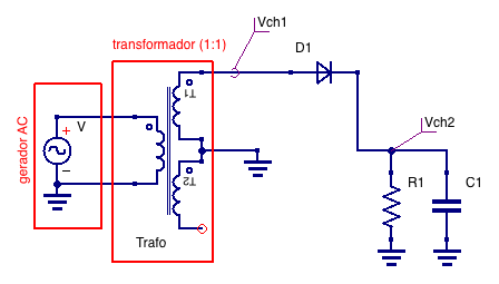
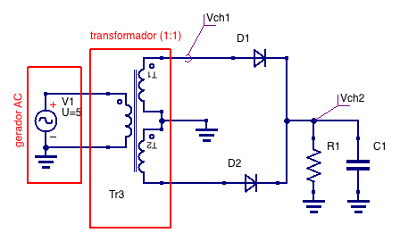
The distribution of electrical energy worldwide is carried out by sine waves, with frequencies in the range of 50−100Hz and amplitudes between 100−300V (within a house). These amplitudes can be reduced by the use of a transformer, but the signal remains alternated, AC. Relative to the neutral wire, these signals exhibit a zero mean or DC value. Most electrical equipment, however, uses continuous power, DC. The transformation of an alternating voltage into continuous voltage is the most important and present application of diodes in our daily lives. The figure below represents the voltage output at the terminals of a transformer, similar to that used in the laboratory. Note that this signal has an average voltage value equal to zero (\(<V(t)>=0\)). Using a diode in a circuit assembly we can obtain a half-wave or full-wave rectification. The following figure shows the full-wave rectification, where the signal coming out of the transformer is rectified.

Fig. 12 Experimental trace of input (left) and half-wave rectified signal (right)

Fig. 13 Experimental trace of input (left) and full-wave rectified signal (right)
Despite the average DC value that appears in the rectified signals, either half-wave of full-wave rectification results in a large ripple (oscillation) of the output voltage.
Filtered rectification
The simplest circuit to minimize the ripples observed in Fig. 12 or Fig. 13 consists of coupling a capacitor to the load, which allows filtering of the ripples and, therefore, minimizing the signal oscillation. The complete model for filter rectification implies an RC circuit, where the signal ripple (ripple voltage) can be expressed by (see section 3.2.3 in [1]):
where \(V_d\approx 0.7\) is the diode voltage drop, and \(\Delta t_{d}\) is the time slot between two successive peaks, i.e., \(\Delta t_{d}\approx T\) for half-wave rectifiers and \(\Delta t_{d}\approx T/2\) for full-wave rectifiers. When \(RC>>\Delta t_{d}\), eq. (15) can be approximated by,
where \(n=1\) (half-wave) or \(n=2\) (full-wave).
Rectified voltage sources
The half-wave rectifier is the simplest voltage source in existence, where only half a cycle of the alternating voltage wave is converted to continuous voltage.
Videos of the experiments
You must login with you @m.unicamp.br account to view these videos!
Half-wave rectifier
This first video illustrate the experimental procedure and data acquisition associated with the half-wave rectifier.
Full-wave rectifier
This second video illustrate the experimental procedure and data acquisition associated with the half-wave rectifier.
#Loading dataset with "tab" as separator
data = pd.read_csv('dados/001_meia_onda_c_R_330.dat',sep='\t')
glue("df_pandas_exemplo_diode_rc", data.head())
| time (s) | CH1 (V) | CH2 (V) | |
|---|---|---|---|
| 0 | 0.00002 | 1.2 | 3.0 |
| 1 | 0.00004 | 1.4 | 3.0 |
| 2 | 0.00006 | 1.4 | 2.8 |
| 3 | 0.00008 | 1.6 | 2.8 |
| 4 | 0.00010 | 1.8 | 3.0 |
Downloadable dataset 1
Two files (.zip):
| time (s) | CH1 (V) | CH2 (V) | |
|---|---|---|---|
| 0 | 0.00002 | 1.2 | 3.0 |
| 1 | 0.00004 | 1.4 | 3.0 |
| 2 | 0.00006 | 1.4 | 2.8 |
| 3 | 0.00008 | 1.6 | 2.8 |
| 4 | 0.00010 | 1.8 | 3.0 |
Fig. 16 Structure of the 001_meia_onda_c_R_330.dat data file, corresponding to the decade resistance at \(330\Omega\); the separator between entries is a tab.
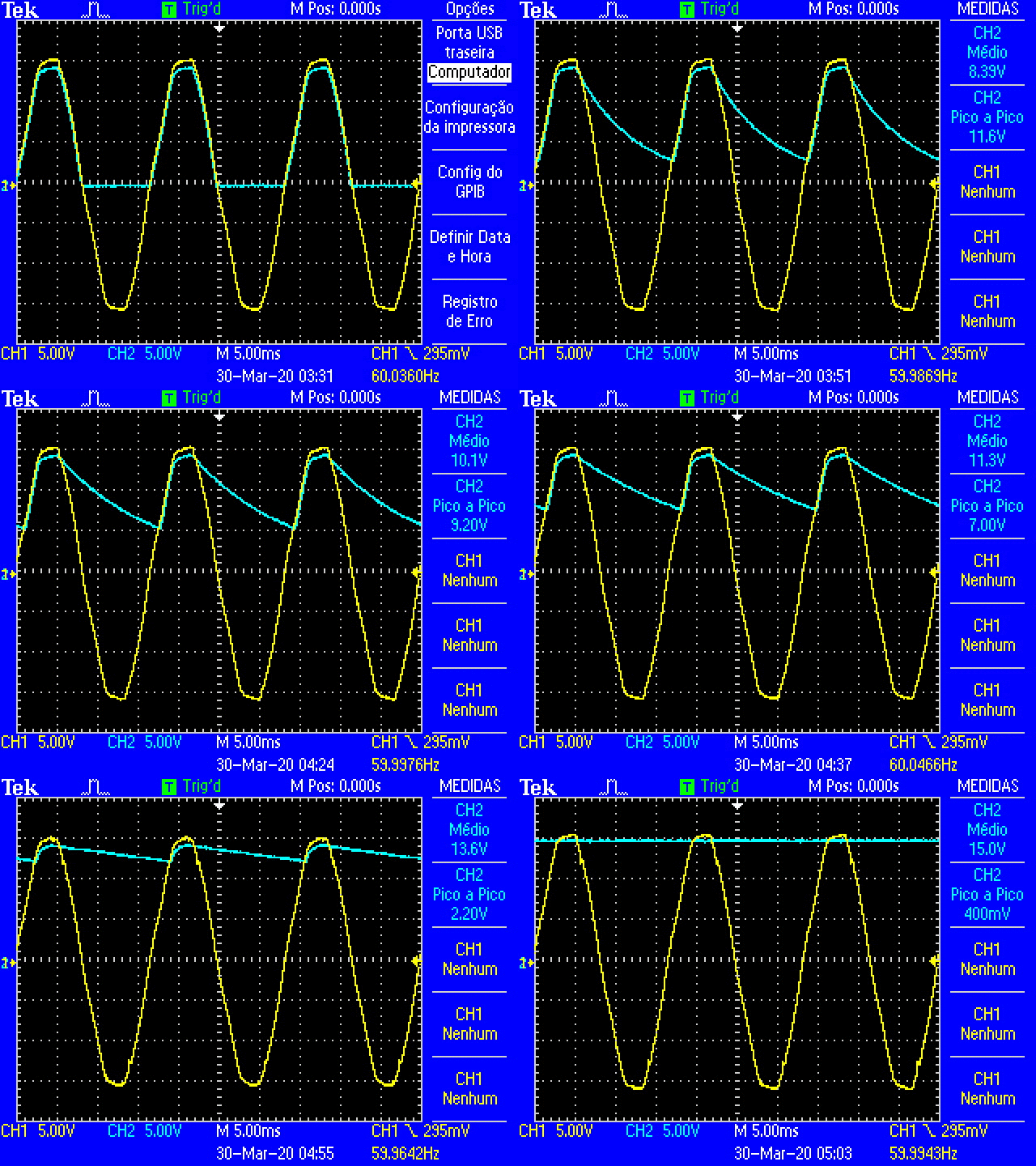
Fig. 17 Oscilloscope traces of the half-wave rectification as the decade resistance is increased.
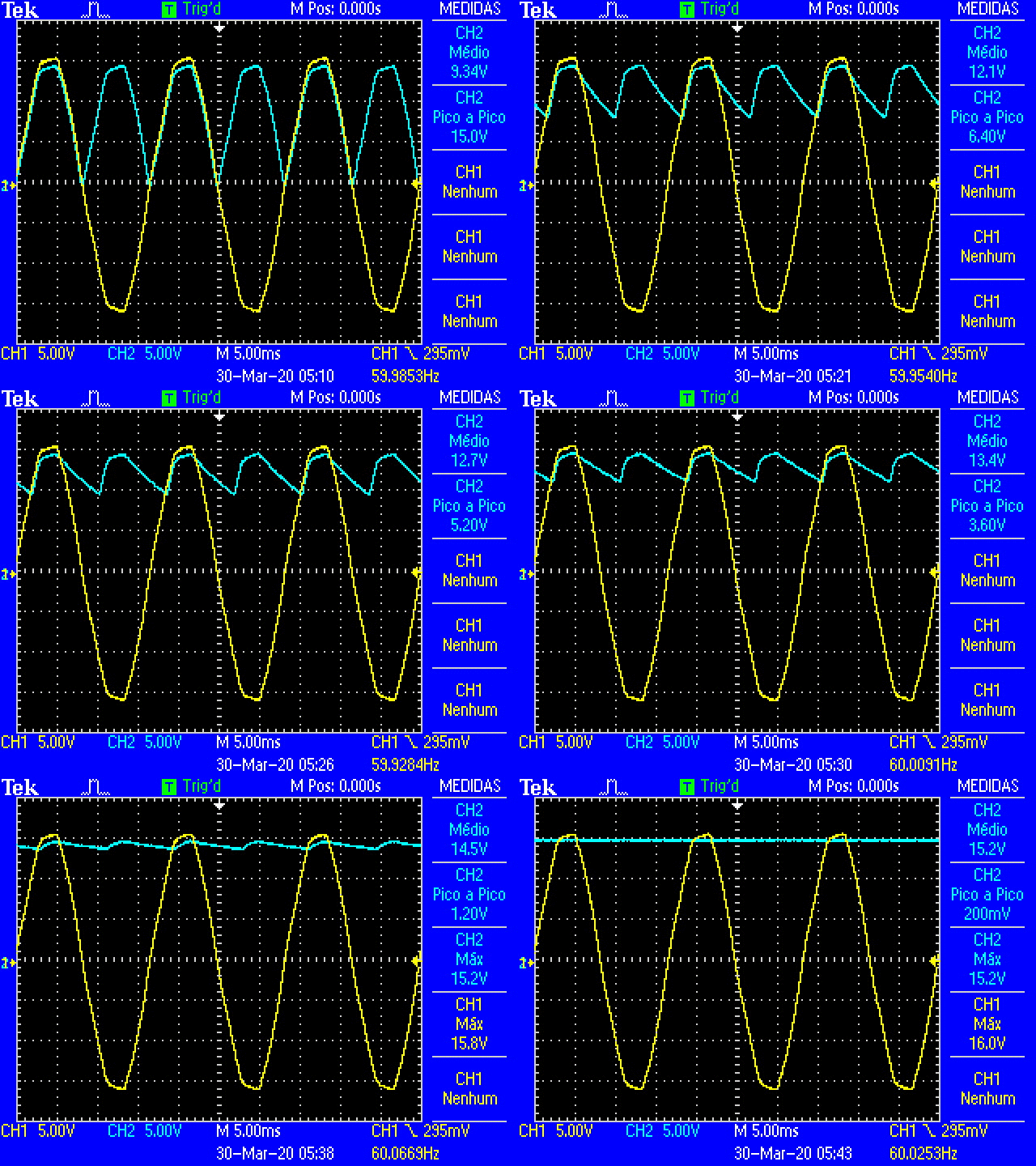
Fig. 18 Oscilloscope traces of the full-wave rectification as the decade resistance is increased.

