Exploring log scale plots with Python¶

Loading packages¶

import numpy as np
import os
import matplotlib.pyplot as plt

#Ajsutando fontes padrão dos gráficos
font = { 'weight' : 'normal',
        'size'   : 16}

plt.rc('font', **font)
#Ajsutando espessura das linhas padrão dos gráficos
plt.rcParams['lines.linewidth'] = 2;

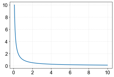
Linear scale¶

Exemplo em que a escala linear é apropriada:¶

npt = 1000 # numero de pontos
x = np.linspace(1e-1,1e1,npt) #vetor linearmente espaçado
y = 1/x 
plt.plot(x,y)
#grades
plt.grid()
#ajustar a razão de aspecto do eixo
plt.show()

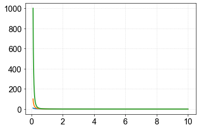
../_images/Plotting - Exploring Log scale_6_0.png

Algumas dificuldades em visualizar propriedades com a escala linear¶

Comparando quantidade com ampla diferença¶

npt = 1000 # numero de pontos
x = np.linspace(1e-1,1e1,npt) #vetor linearmente espaçado
for n in [1,2,3]:
    y = 1/x**n 
    plt.plot(x,y)
#grades
plt.grid()
#ajustar a razão de aspecto do eixo
plt.show()

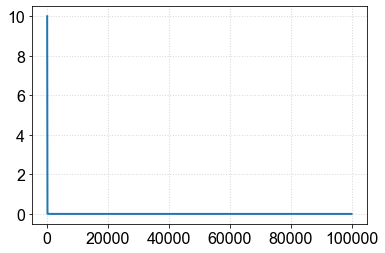
../_images/Plotting - Exploring Log scale_9_0.png

Eixo horizontal cobrindo ampla faixa de valores¶

npt = 1000 # numero de pontos
x = np.linspace(1e-1,1e5,npt) #vetor linearmente espaçado
y = 1/x 
plt.plot(x,y)
#grades
plt.grid()
#ajustar a razão de aspecto do eixo
plt.show()

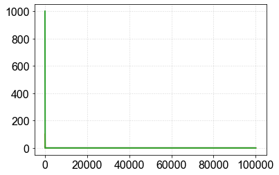
../_images/Plotting - Exploring Log scale_11_0.png

Fica ainda pior quando se tenta comparar diferentes funções¶

npt = 1000 # numero de pontos
x = np.linspace(1e-1,1e5,npt) #vetor linearmente espaçado
for n in [1,2,3]:
    y = 1/x**n 
    plt.plot(x,y)
#grades
plt.grid()
#ajustar a razão de aspecto do eixo
plt.show()

../_images/Plotting - Exploring Log scale_13_0.png

How about using the log function to improve this aspect of the visualization?¶

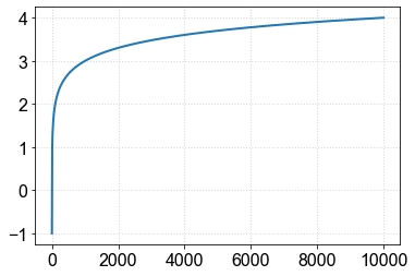
The log function¶

npt = 1000 # numero de pontos
x = np.linspace(1e-1,1e4,npt) #vetor linearmente espaçado
y = np.log10(x)
plt.plot(x,y)
#grades
plt.grid()

../_images/Plotting - Exploring Log scale_16_0.png

Two ways to plot in log scale:¶

draw an axis with logarithmic spacing: \( x '= \ log10 (x) \)
perform the variable transformation of the original axis coordinate (\(x\)) to a new coordinate (\(x'\)):

(3)¶\[ x = 10 ^ {x '} \]

Determining the position of tickmarks in a log plot¶

xvec = np.array([0.01, 0.1, 1,10, 100])
xlog_ticks1 = np.log10(xvec)
print('tick position1:',xlog_ticks1)
#------
xvec = 2*np.array([0.01,0.1, 1,10])
xlog_ticks2 = np.log10(xvec)
print('tick position2:',xlog_ticks2)
#------
xvec = 3*np.array([0.01,0.1, 1,10])
xlog_ticks3 = np.log10(xvec)
print('tick position3:',xlog_ticks3)
#------
xvec = 5*np.array([0.01,0.1, 1,10])
xlog_ticks5 = np.log10(xvec)
print('tick position5:',xlog_ticks5)

tick position1: [-2. -1.  0.  1.  2.]
tick position2: [-1.69897 -0.69897  0.30103  1.30103]
tick position3: [-1.52287875 -0.52287875  0.47712125  1.47712125]
tick position5: [-1.30103 -0.30103  0.69897  1.69897]

#criando grade do gráfico
fig,ax = plt.subplots(figsize=(12,8))
#
# #pontos na posição dos "ticks" x'=log10(x)
# plt.plot(xlog_ticks1,0*xlog_ticks1,'ro')
# #---
# #linhas na posição dos "ticks" x'=log10(x)
# for x0 in xlog_ticks1:
#     plt.axvline(x0,linestyle='--',color='r')
# #---
# #refinando os ticks  - multiplos de 2
# plt.plot(xlog_ticks2,0*xlog_ticks2,'b*')    
# for x0 in xlog_ticks2:
#     plt.axvline(x0,linestyle='-.',color='b')
# #--
# #refinando os ticks  - multiplos de 3
# plt.plot(xlog_ticks3,0*xlog_ticks3,'g*')    
# for x0 in xlog_ticks3:
#     plt.axvline(x0,linestyle='-.',color='g')
# #--
# #refinando os ticks  - multiplos de 5
# plt.plot(xlog_ticks5,0*xlog_ticks3,'m*')   
# for x0 in xlog_ticks5:
#     plt.axvline(x0,linestyle='-.',color='m')
#--------
#formatacao
#grades
plt.grid()
xrange, yrange = 2,2
xstep, ystep = 0.5,1
plt.xlim([-xrange-0.1,xrange+0.1])
plt.ylim([-yrange-0.1,yrange+0.1])
plt.xticks(np.arange(-xrange,xrange+1,xstep))
plt.yticks(np.arange(-yrange,yrange+1,ystep))
plt.show()

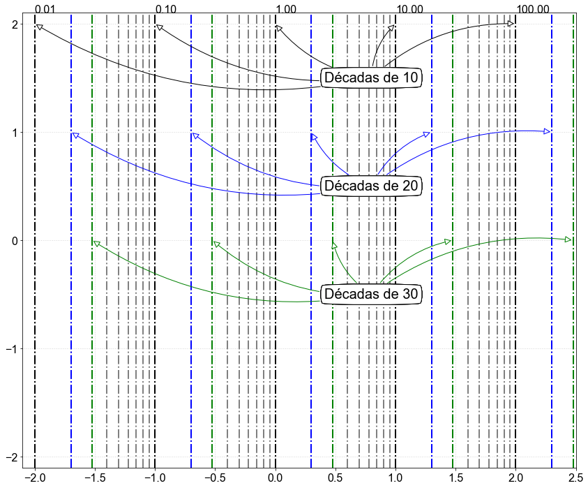
../_images/Plotting - Exploring Log scale_20_0.png

Generating markers and annotations¶

#criando grade do gráfico
fig,ax = plt.subplots(figsize=(12,10))
#
#pontos na posição dos "ticks" x'=log10(x)

#---
xvec = np.array([0.01, 0.1, 1,10, 100])
#linhas na posição dos "ticks" x'=log10(x)
for multiplo in [1,2,3,4,5,6,7,8,9]:
    xlog_ticks = np.log10(multiplo*xvec)
    x_ticks = multiplo*xvec
    #-verticais
    for x0,xlin in zip(xlog_ticks,x_ticks):
        plt.axvline(x0,linestyle='-.',color='gray')
#-----------------
#decadas de  10
for multiplo in [1,]:
    xlog_ticks = np.log10(multiplo*xvec)
    x_ticks = multiplo*xvec
    #-verticais
    for x0,xlin in zip(xlog_ticks,x_ticks):
        plt.axvline(x0,linestyle='-.',color='k')
    #-verticais
    for x0,xlin in zip(xlog_ticks,x_ticks):
        ax.annotate('{:0.2f}'.format(10**(x0)), xy=(x0, 2.1),) 
        ann1 = ax.annotate("Décadas de 10",
                  xy=(x0, 2), xycoords='data',
                  xytext=(0.8,1.5), textcoords='data',
                  size=20, va="center", ha="center",
                  bbox=dict(boxstyle="round4", fc="w"),
                  arrowprops=dict(arrowstyle="-|>",
                                  connectionstyle="arc3,rad=-0.2",
                                  fc="w"),
                  )
#-----------------
#decadas de  20
for multiplo in [2,]:
    xlog_ticks = np.log10(multiplo*xvec)
    x_ticks = multiplo*xvec
    for x0,xlin in zip(xlog_ticks,x_ticks):
        plt.axvline(x0,linestyle='-.',color='b')
    #-verticais
    for x0,xlin in zip(xlog_ticks,x_ticks):
        ann1 = ax.annotate("Décadas de 20",
                  xy=(x0, 1), xycoords='data',
                  xytext=(0.8,0.5), textcoords='data',
                  size=20, va="center", ha="center",
                  bbox=dict(boxstyle="round4", fc="w"),
                  arrowprops=dict(arrowstyle="-|>",
                                  connectionstyle="arc3,rad=-0.2",
                                  fc="w",color='blue'),
                  )
#-----------------
#decadas de  30
for multiplo in [3,]:
    xlog_ticks = np.log10(multiplo*xvec)
    x_ticks = multiplo*xvec
    for x0,xlin in zip(xlog_ticks,x_ticks):
        plt.axvline(x0,linestyle='-.',color='g')
    #-verticais
    for x0,xlin in zip(xlog_ticks,x_ticks):
        ann1 = ax.annotate("Décadas de 30",
                  xy=(x0, 0), xycoords='data',
                  xytext=(0.8,-0.5), textcoords='data',
                  size=20, va="center", ha="center",
                  bbox=dict(boxstyle="round4", fc="w"),
                  arrowprops=dict(arrowstyle="-|>",
                                  connectionstyle="arc3,rad=-0.2",
                                  fc="w",color='g'),
                  )
#--------
#formatacao
#grades
plt.grid()
xrange, yrange = 2,2
xstep, ystep = 0.5,1
plt.xlim([-xrange-0.1,xrange+0.1])
plt.ylim([-yrange-0.1,yrange+0.1])
plt.xticks(np.arange(-xrange,xrange+1,xstep))
plt.yticks(np.arange(-yrange,yrange+1,ystep))
plt.tight_layout()
plt.show()

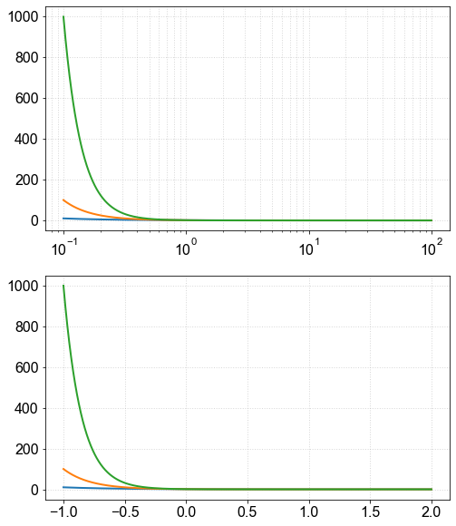
../_images/Plotting - Exploring Log scale_22_0.png

Exemplo com eixo x (using `plt.semilogx()`):¶

\(x'=\log_{10}(x)\)

fig,ax = plt.subplots(2,1,figsize=(8,10))
#---------------------------------
#METODO 1, RECOMENDADO, USE AS FUNÇÕES SEMILOGX OU SEMILOGY OU LOGLOG
npt = 100000 # numero de pontos
xmin = 1e-1
xmax = 1e2
x = np.linspace(1e-1,1e2,npt) #vetor linearmente espaçado
ax0 = ax[0]
for n in [1,2,3]:
    y = 1/x**n 
    ax0.semilogx(x,y)
#----------------------------------
#METODO 2, RECOMENDADO, USE AS FUNÇÕES SEMILOGX OU SEMILOGY OU LOGLOG
npt = 100000 # numero de pontos
x1min = np.log10(xmin)
x1max = np.log10(xmax)
x1 = np.linspace(x1min,x1max,npt) #vetor linearmente espaçado na coordenada x1
ax0 = ax[1]
for n in [1,2,3]:
    y = 1/10**(n*x1)
    ax0.plot(x1,y)
#grades
ax[0].grid(True,which='Both')
ax[1].grid()
plt.show()

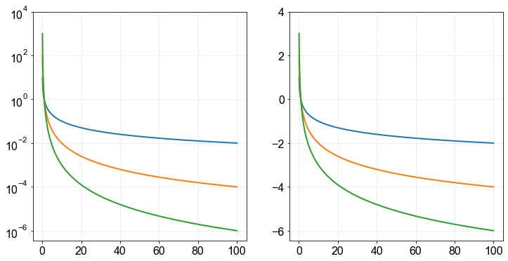
../_images/Plotting - Exploring Log scale_25_0.png

Exemplo com eixo y (using `plt.semilogy()`)¶

\(y'=\log_{10}(y)\)

fig,ax = plt.subplots(1,2,figsize=(12,6))
#---------------------------------
#METODO 1, RECOMENDADO, USE AS FUNÇÕES SEMILOGX OU SEMILOGY OU LOGLOG
npt = 100000 # numero de pontos
xmin = 1e-1
xmax = 1e2
x = np.linspace(1e-1,1e2,npt) #vetor linearmente espaçado
ax0 = ax[0]
for n in [1,2,3]:
    y = 1/x**n 
    ax0.semilogy(x,y)
ax0.set_yticks([1e-6,1e-4,1e-2,1,1e2,1e4])
#----------------------------------
#METODO 1, RECOMENDADO, USE AS FUNÇÕES SEMILOGX OU SEMILOGY OU LOGLOG
npt = 100000 # numero de pontos
# x1min = 10**(xmin)
# x1max = 10**(xmax)
ax0 = ax[1]
for n in [1,2,3]:
    y1 = -n*np.log10(x) 
    ax0.plot(x,y1)
ax0.set_yticks([-6,-4,-2,0,2,4])
#grades
ax[0].grid()
ax[1].grid()
plt.show()

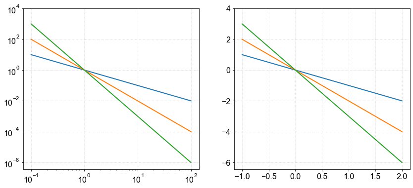
../_images/Plotting - Exploring Log scale_27_0.png

Examples with two axes, x,y (using `plt.loglog()`):¶

\(x'=\log_{10}(x)\)

\(y'=\log_{10}(y)\)

fig,ax = plt.subplots(1,2,figsize=(14,6))
#---------------------------------
#METODO 1, RECOMENDADO, USE AS FUNÇÕES SEMILOGX OU SEMILOGY OU LOGLOG
npt = 100000 # numero de pontos
xmin = 1e-1
xmax = 1e2
x = np.linspace(1e-1,1e2,npt) #vetor linearmente espaçado
ax0 = ax[0]
for n in [1,2,3]:
    y = 1/x**n 
    ax0.loglog(x,y)
ax0.set_yticks([1e-6,1e-4,1e-2,1,1e2,1e4])
#----------------------------------
#METODO 1, RECOMENDADO, USE AS FUNÇÕES SEMILOGX OU SEMILOGY OU LOGLOG
npt = 100000 # numero de pontos
x1min = np.log10(xmin)
x1max = np.log10(xmax)
x1 = np.linspace(x1min,x1max,npt) #vetor linearmente espaçado na coordenada x1
ax0 = ax[1]
for n in [1,2,3]:
    y1 = -n*x1
    ax0.plot(x1,y1)
ax0.set_yticks([-6,-4,-2,0,2,4])
#grades
ax[0].grid()
ax[1].grid()
plt.show()

../_images/Plotting - Exploring Log scale_29_0.png

Linearization examples¶

It is also possible to directly transform the variables to a log scale using (3) , and use the regular plt.plot() function. It is important, however, to pay attention to the following issues:

Do not take logarithm of null or negative quantities, they will either diverge or result in complex numbers
Make sure you have dimensionless quantities before taking the log scale, otherwise you end up with meaningless units, such as \(\log(Hz)\).

For example, if the axis \(x\) to be transformed is in units of \([m]\), before using (3) you can pick an appropriate reference value, say \(1 m\) and normalize your axis relative to that: \(x\rightarrow\frac{x}{1m}\). The label of your axis in this case would be \(\log(\frac{x}{m})\). For instance, after normalization, if a given point along the transformed axis (\(x`=\log(x)\)) has a value of \(x'=3.2'\), then \(\frac{x}{m}=10^{3.2}\approx1584.9\) and \(x\approx1584.9m\).

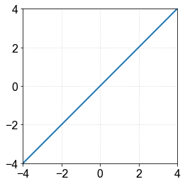
a) Seja \(y(x)=x\). Qual a inclinação da reta em escala log?¶

npt = 1000 # numero de pontos
x = np.linspace(1e-4,1e4,npt) #vetor linearmente espaçado
y = x
#
xlog = np.log10(x)
ylog = np.log10(y)
#
plt.plot(xlog,ylog)
#grades
plt.grid()
#ajustar a razão de aspecto do eixo
plt.ylim([-4,4])
plt.xlim([-4,4])
ax = plt.gca()
ax.set_aspect(aspect=1)
plt.show()

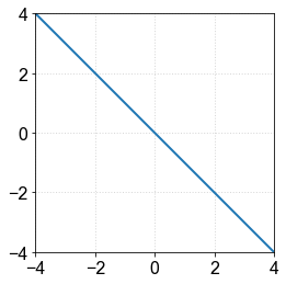
../_images/Plotting - Exploring Log scale_32_0.png

b) Seja \(y(x)=x^{-1}\). Qual a inclinação da reta em escala log?¶

npt = 1000 # numero de pontos
x = np.linspace(1e-4,1e4,npt) #vetor linearmente espaçado
y = 1/x
#
xlog = np.log10(x)
ylog = np.log10(y)
#
plt.plot(xlog,ylog)
#grades
plt.grid()
#ajustar a razão de aspecto do eixo
plt.ylim([-4,4])
plt.xlim([-4,4])
ax = plt.gca()
ax.set_aspect(aspect=1)
plt.show()

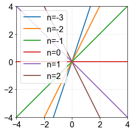
../_images/Plotting - Exploring Log scale_34_0.png

b) What happens when the polynomial has other powers? i.e., \( y(x) = x^n \)¶

npt = 1000 # numero de pontos
x = np.linspace(1e-4,1e4,npt) #vetor linearmente espaçado
#---
for n in range(-3,3):
    y = 1/x**n # n é a potência do polinômia
    #
    xlog = np.log10(x)
    ylog = np.log10(y)
    #
    plt.plot(xlog,ylog,'-',label='n={:1}'.format(n))
#grades
plt.grid()
#ajustar a razão de aspecto do eixo
plt.ylim([-4,4])
plt.xlim([-4,4])
ax = plt.gca()
ax.set_aspect(aspect=1)
plt.legend(loc='best')
plt.show()

../_images/Plotting - Exploring Log scale_37_0.png

É importante usar espaçamento logarítmico dos pontos!

F540 Interactive Book